source("https://raw.githubusercontent.com/ChrisWudel/Multi-trait-point-pattern-reconstruction/main/func/setup.R")

setup(
  packages = c("spatstat", "ggplot2"),
  func_names = c("reconstruct_pattern_multi", "compute_statistics",
                 "dummy_transf", "energy_fun", "calc_moments", "select_kernel",
                 "plot.rd_multi", "sample_points", "edge_correction", "vis_patterns")
)4 Specialized application
This represents a novel workflow for predicting forest regeneration. Initially, the canopy of a forest area and a small portion of the regeneration were captured using terrestrial laser scanning. Based on spatial statistical tree data and correlations between tree characteristics, a point pattern reconstruction method was developed, building upon the work of Wudel et al. (2023). This method facilitates the prediction of regeneration across the entire area with high accuracy.
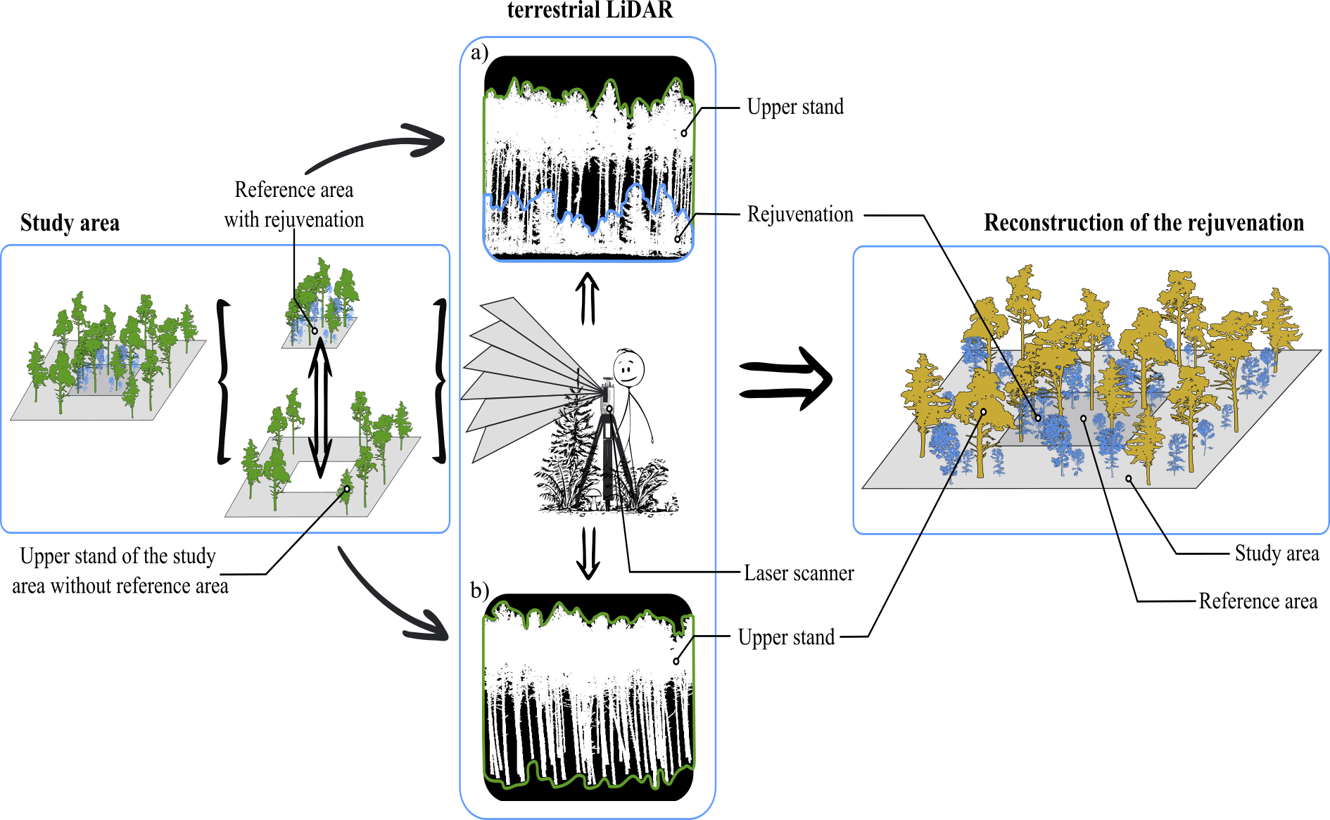
Figure: Conceptual presentation of the new innovative workflow for data acquisition and reconstruction of forest regeneration (LiDAR = Light Detection and Ranging). a) Recording regeneration on a small area and b) recording of the upper stand trees at the whole forest area.
The following code can be used to execute the workflow using an available dataset. First, the necessary functions and packages are loaded.
Subsequently, the dataset is retrieved from the ‘Records’ folder on GitHub and published and freely available at the following link: https://zenodo.org/records/10550778 (Meyer and Wudel, 2024).
url <- "https://raw.githubusercontent.com/ChrisWudel/Multi-trait-point-pattern-reconstruction/main/Records/Real_datasets/Terrestrial_laser_scan_data_340_a31.csv"
data <- read.csv(url,sep = ",", stringsAsFactors= TRUE)
data$dbh <- as.numeric(data$dbh)

data <- data.frame(data[2],data[3],data[4],data[5])
colnames(data) <- c("x", "y", "dbh", "species")
Below are the parameter settings chosen for this example. These may and should be adjusted for other datasets to achieve good results. Note: the maximum number of steps has also been reduced here to limit computation time.
W <- owin(c(0, 100),c(0, 100))
core_window <- owin(c(35, 65),c(35, 65))

marked_pattern <- as.ppp(data.frame(data), W = W)
marked_pattern$marks$dbh <- marked_pattern$marks$dbh*0.001
xr <- marked_pattern$window$xrange
yr <- marked_pattern$window$yrange
obs_window = owin(c(xr),c(yr))

reconstruction <- reconstruct_pattern_multi(
marked_pattern,
fixed_points      = NULL,
edge_correction   = TRUE,
n_repetitions     = 1,
max_steps         = 10000,
no_change         = 5,
rcount            = 250,
rmax              = 25,
issue             = 5000,
divisor           = "r",
kernel_arg        = "epanechnikov",
timing            = TRUE,
energy_evaluation = TRUE,
show_graphic      = FALSE,
Lp                = 1,
bw                = 0.5,
sd                = "step",
steps_tol         = 10000,
tol               = 1e-4,
w_markcorr        = c(m_m=0,one_one=1500,  all=1, m_all=1, all_all=1, m_m0=1500, one_one0=1, all0=1, m_all0=1, all_all0=1),
prob_of_actions   = c(move_coordinate = 0.3, switch_coords = 0.1, exchange_mark_one = 0.1, exchange_mark_two = 0.1, pick_mark_one = 0.1, pick_mark_two = 0.1, delete_point = 0.1, add_point = 0.1),
k                 = 1,
w_statistics      = c(),
is.fixed          = function(p) 35 <= p$x & p$x <= 65 & 35 <= p$y & p$y <= 65 | p$mark[,"dbh"] > 0.1,
verbose           = TRUE)
> Progress:  || iterations: 0 || Simulation progress: 0% || energy = 28.36318 || energy improvement = 0
> Progress:  || iterations: 5000 || Simulation progress: 50% || energy = 12.84772 || energy improvement = 88
> Progress:  || iterations: 10000 || Simulation progress: 100% || energy = 8.25349 || energy improvement = 119
The following figure shows the results of the workflow, which are from an example not derived from the current run. The figure has been created retroactively and is not generated by the function provided. Additionally, in this simulation, significantly more simulation steps were conducted, which would take too long to render for this handbook.
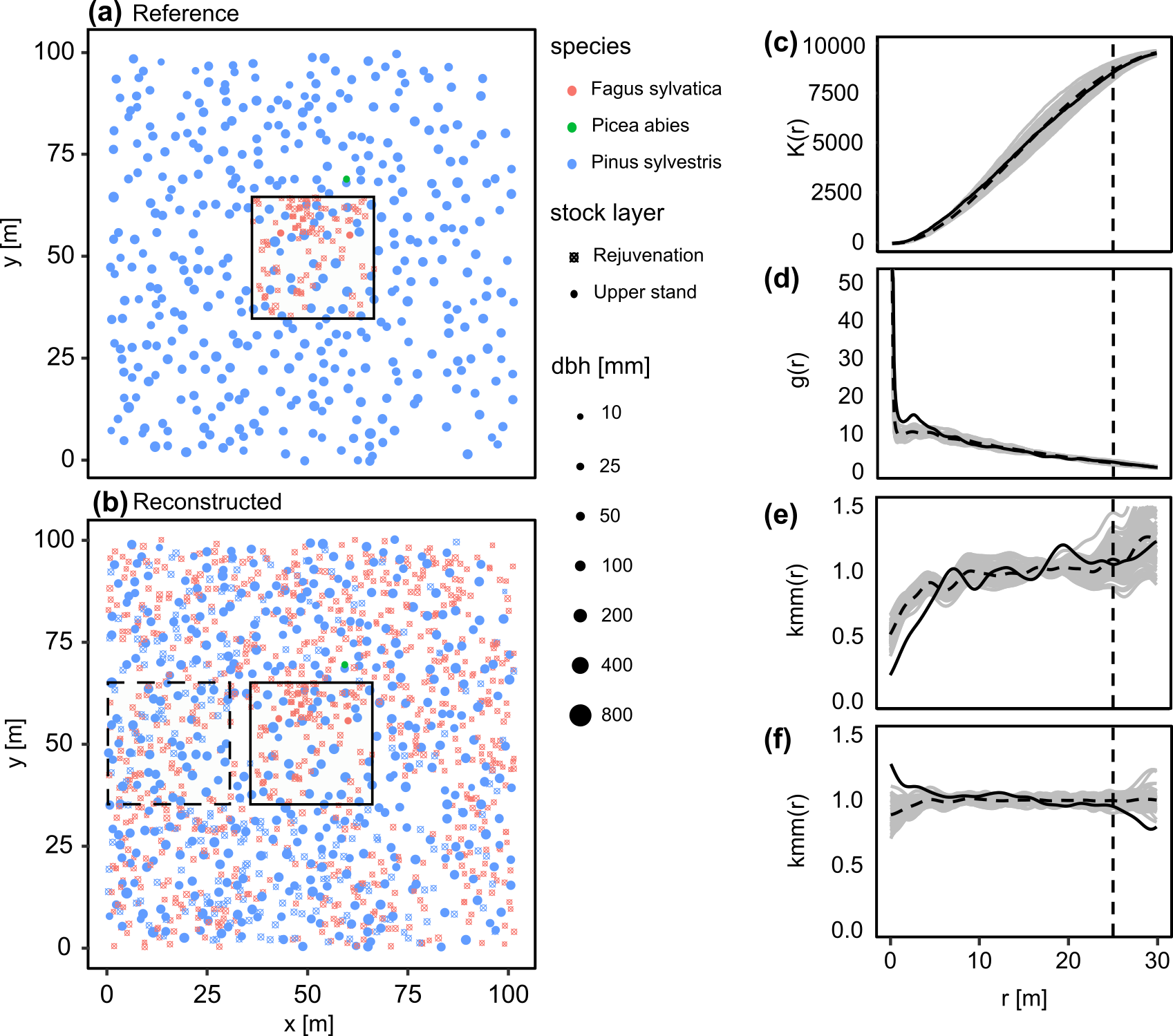
Figure: Results of the 100 reconstructions of the dataset described above; (a) reference pattern with core area, black outlined area (b) an example of a reconstruction in which the core area is outlined in black and the comparison area is outlined in black dashed lines. Summary statistics (c)–(f) were generated using the R package ‘spatstat’: (c) K function; (d) pcf; (e) mcf of the species, where the test function has value if both species coincide and if not; (f) mcf of the diameter, the test function being the usual product. For distances up to = 25 m (indicated by the vertical dashed line in (c)–(f)). The black solid lines represent the reference curve and the grey solid lines represent the 100 reconstructions. The dashed black line is the mean of the 100 reconstructions.
It is evident that the tree distributions in these two areas are similar. For instance, Fagus sylvatica is observed with high intensity only in specific regions of the reference area, and this has been successfully reproduced. Furthermore, it is noticeable that smaller gaps in the reference area, where canopy trees are spaced similarly, are not occupied by regeneration plants in the comparison area. Also includes the previously mentioned summary statistics of all 100 reconstructions (c)-(f). These statistics demonstrate that the reconstructions perform well (gray lines = reconstructions, solid black line = reference). Within the range up to 25 m, which was considered during reconstruction, deviations from the reference in the K-function (c) are minimal. The pcf (d) shows a slight systematic deviation. The mcf of the species (e) exhibit only minimal discrepancies. The mcf of diameters (f) show smaller discrepancies in the same close range as the pcf. However, deviations become significantly larger and more diverse once the 25 m range is exceeded. This highlights the effectiveness and impact of the mcf’s in the reconstruction method.