source("https://raw.githubusercontent.com/ChrisWudel/Multi-trait-point-pattern-reconstruction/main/func/setup.R")

setup(
  packages = c("spatstat", "ggplot2", "patchwork"),
  func_names = c("reconstruct_pattern_multi", "compute_statistics",
                 "dummy_transf", "energy_fun", "calc_moments", "select_kernel",
                 "plot.rd_multi", "sample_points", "vis_patterns", "select_data")
)3 Further application examples
In the following, further examples of the simple application of Multi-Trait Point Pattern Reconstruction (MTPPR) presented in Wudel et al. (2023) are presented. These are standard applications, meaning that reconstructions are performed without enlargements or reductions of the reconstruction pattern and without edge correction.
First, the necessary functions and packages will be loaded. If individual R packages are not installed, install them as follows: install.packages("package name").
Now you need to define which dataset you want to use. There are 2 real datasets and 4 generated datasets available. To select a dataset, define x with the name of the dataset you want to use (x <- ‘Dataset Name’). The datasets are available under ’Records for download.
x <- "random" ## The following sets can be imported:
                                   ## Real datasets:
                                    ##    "VERMOS_project"
                                    ##    "Northwest_German_Forest_Research_Institute"
                                    ##   "Marteloscope_data_from_the_by_the_Chair_of_Forest_Growth_and_Woody_Biomass_Production"
                                   ## Simulated patterns:
                                    ##    "random"
                                    ##    "regular"
                                    ##    "cluster_size5"
                                    ##    "cluster_size5_and_random"
                                   ## to do this, declare x with the corresponding name in "".
data <- data_import(x)
W <- data[[2]]
data <- data [[1]]
The following parameters are predefined and can be varied arbitrarily in an application file (Application of the Multi-trait Point pattern reconstruction.R) where you can use this code, available for download under the Application folder. It should be noted that for optimal results, the parameter max_steps should be at least approximately ten times the number of points in the pattern, and the parameter for weights (w_markcorr) of individual summary statistics needs to be adjusted according to different scenarios. Here, a small number of steps was chosen to save computation time.
marked_pattern <- as.ppp(data.frame(data), W = W)
marked_pattern$marks$dbh..mm.<-marked_pattern$marks$dbh..mm.*0.001
xr <- marked_pattern$window$xrange
yr <- marked_pattern$window$yrange

reconstruction <- reconstruct_pattern_multi(
  marked_pattern,
  n_repetitions     = 1,
  max_steps         = 10000,
  no_change         = 5,
  rcount            = 250,
  rmax              = 25,
  issue             = 1000,
  divisor           = "r",
  kernel_arg        = "epanechnikov",
  timing            = TRUE,
  energy_evaluation = TRUE,
  show_graphic      = FALSE,
  Lp                = 1,
  bw                = 0.5,
  sd                = "step",
  steps_tol         = 1000,
  tol               = 1e-4,
  w_markcorr        = c(m_m=1,one_one=0,  all=1, m_all=1, all_all=1, m_m0=1, one_one0=0, all0=1, m_all0=1, all_all0=1),
  prob_of_actions   = c(move_coordinate = 0.4, switch_coords = 0.1, exchange_mark_one = 0.1, exchange_mark_two = 0.1, pick_mark_one = 0.2, pick_mark_two = 0.1, delete_point = 0.0, add_point = 0.0),
  k                 = 1,
  w_statistics      = c(),
  verbose           = TRUE)
As a result, you will receive a list with a variety of information, such as the reference pattern, the reconstructed pattern, the number of successful actions, the energy development, and much more. To illustrate the results, first compare the reference pattern with the reconstructed pattern.
vis_pp(reconstruction) [1] "look under Plots to see the result."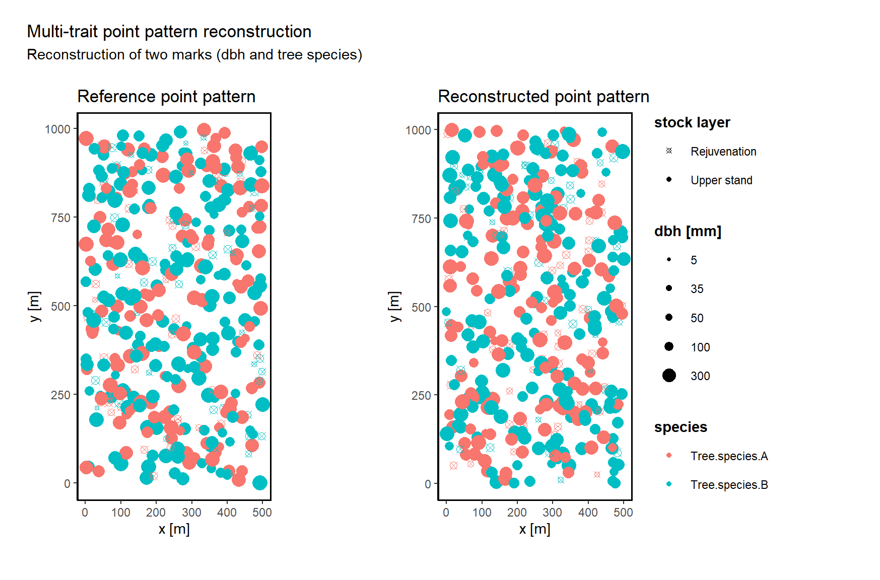
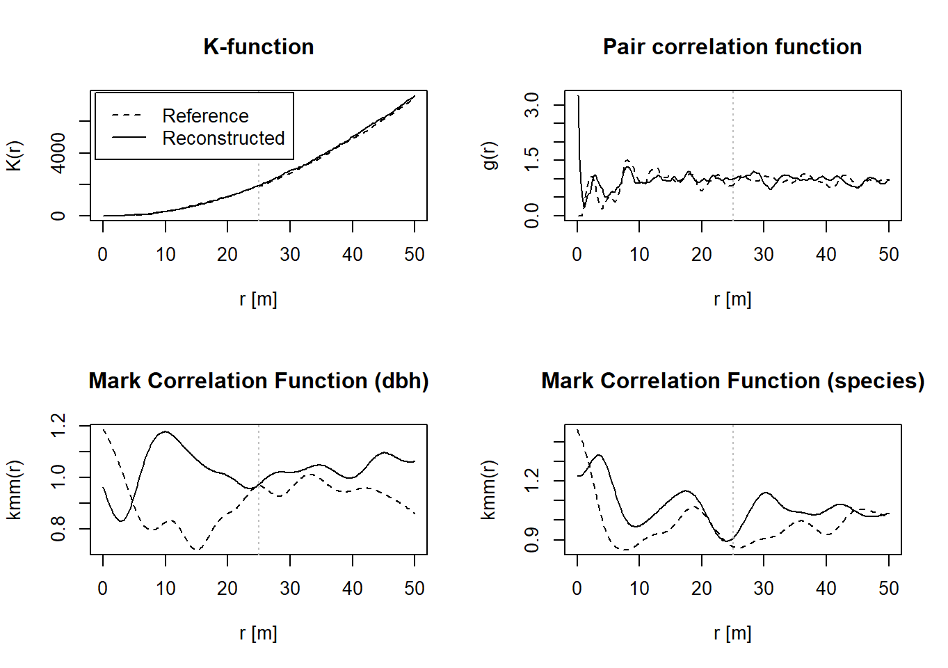
Finally, you can use the following function to compare various summary statistics of the reference pattern (black line) with the reconstructed pattern (grey line). Another function (plot_sum_stat) is capable of displaying these summary statistics in a single diagram for multiple repetitions of the reconstructions (n_repetitions > 1), and it is used in the previously mentioned application file (Application of the Multi-trait Point pattern reconstruction.R). For simplicity, this functionality has been omitted here.
plot(reconstruction)